What do skateboarders talk about?

It turns out, mostly skateboarding, videos, teams, and people named Mike.

To find out, I analyzed over 50 interviews from the wonderful skateboarding blog the chrome ball incident.  I did this by scraping the content from the site (with python, of course) and then filtering out some common words (stop words) to get meaningful results.  I then used Wordle (which is really, really cool) to make tag clouds of the 150 most frequently used words in all of the interviews.

The total word count was a whopping 229,199 words (for comparison).  The first round of filtering was pretty modest - I only removed the 186 most commonly used English words.  Here are the results (click the photo to embiggen):

skate_text1_wm
Including a slightly larger list of stop words reveals a bit more character:

skate_text2_wm

Amongst the expletives and common skate-slang ('dude', 'stoked', 'rad', 'spot', etc.), the word 'street' (as in, street skating) is mentioned 3 times as frequently as 'vert' (as in, vert skating) - something we've seen before.

You can see the raw data here and here for each stop word filtering.  Play with it please!

The physics of Jake Brown's ollie 720

I'm a couple weeks late on this, but recently Jake Brown landed the first ever ollie 720.  To put that in layman's terms, he did two full rotations without holding the board on his feet with his hands.  Check it out:


So this seems crazy.  How did he do that?  How did he keep the board on his feet?  Magnets?  It turns out, it's actually very simple physics:

The Conservation of Energy


That's it!  Jake Brown doesn't really have to do anything because the conservation of energy won't be violated (it's a law!).  So yeah, thanks physics!  Skateboarding is so easy.


New project: wools++

I've taken on another minecraft related project in an attempt to learn some more python as well as some basic web development.


Introducing wools++

Centered on the Overcast Network (formerly Project Ares) collection of minecraft servers, wools++ collects data from a user's profile a few times per day and produces more sophisticated statistics (such as rolling values) and even some time series plots.  Here's a couple from my profile:

kd
rkd


With:

  • KD = kills/deaths
  • RK7 = rolling kills (kills over the last 7 days)
  • RD7 = rolling deaths
  • RKD7 = rolling KD

The name itself comes from a capture-the-flag type game often played on the servers, where the flag is replaced by a minecraft wool block.  If you successfully capture a wool block, your "wools" count is incremented.

The project is hosted on Google's app engine for a couple reasons.

  • It can be free (if your app is small enough)
  • Built in datastore (no need to worry about setting up my own SQL database or anything)
  • Python support.  This is great because python is generally a super useful language to know, particularly in the computational sciences.

In the future I'll definitely spend some time discussing the process I went through building this app, because in some cases Google's documentation was a little bit light on the details.  For now, check out the about page if you'd like to read about more details, and you can find the source here.


Pretty Graph of the Day, Part II

solutionSnap

I like this series of graphs because it looks like someone is pulling on the solution like it's a string, until SNAP!  What's being shown here is the numerical solution to the initial value problem

, , .

As you might suspect from the denominator, there's trouble when .  This results in a problem that's not well-posed.  Using the same numerical scheme but only a different number of grid points produces wildly different behaviors.  What's basically happening is that if the numerical scheme hits the trouble region "just right" due to the grid point spacing, the gigantic derivative sends the solution flying off to some large and incorrect value.

You can reproduce this figure in Mathematica with the following code:

1
2
3
4
5
6
7
8
9
10
11
12
13
14
15
16
17
18
19
20
21
22
23
24
25
26
27
28
29
30
31
32
33
34
35
36
37
38
39
(* 4th Order Runge-Kutta Method *)
rungeKutta[y0_, npoints_, a_, b_, f_] := (
   h = (b - a)/(npoints - 1);
   y = Table[0, {npoints}];
   t = Table[0, {npoints}];
   y[[1]] = y0;
   t[[1]] = a;
   Do[
    yn = y[[n]];
    tn = t[[n]];
    m1 = f[tn, yn];
    m2 = f[tn + 0.5*h, yn + 0.5*h*m1];
    m3 = f[tn + 0.5*h, yn + 0.5*h*m2];
    m4 = f[tn + h, yn + h*m3];
    y[[n + 1]] = yn + (1/6)*h*(m1 + 2*m2 + 2*m3 + m4);
    t[[n + 1]] = tn + h;
    , {n, 1, npoints - 1}];
   solution = Table[{t[[i]], y[[i]]}, {i, 1, Length[t]}];
   Return[solution];
   );
 
 f[t_, y_] := 1/(y - 1)^2
y0 = 0;
a = 0; (* Starting t *)
b = 1; (* Ending t *)
 
rks = {};
Do[
  npoints = 10^5 + i; (* Number of grid points *) 
  sol = rungeKutta[y0, npoints, a, b, f];
  p = ListPlot[sol, PlotStyle -> {PointSize[0.001] , Orange}, 
    Frame -> True, AxesLabel -> {"t", "y"}, 
    PlotLabel -> 
     "10^5+ " <> ToString[i] <> 
      " grid points"];
  AppendTo[rks, p];
  , {i, 0, 4}];
 
GraphicsColumn[Table[rks[[j]], {j, 5}], Frame -> All, ImageSize -> 300]

It'll probably take several seconds to run because of the large number of grid points used in each solution.

Video Game Math: KD Ratio Lag

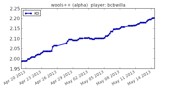
A very common statistic in video games is the kills-to-deaths ratio (KD), which is computed as the number kills divided by the number deaths you've achieved in the game.  The KD is very popular in first person shooters, but can be found in most any place where there's player vs. player combat.  Your KD can be interpreted as the number of kills you tend to get for each death you accumulate (environmental or otherwise).  As you play your game of choice you (hopefully) get better with time, which is reflected in your increasing KD.  However, you may have noticed that the rate at which your KD increases slows down over time (KD lag).  Let’s see why.

First let’s figure out how much your KD increases when adding kills.


Let be your new KD after adding kills to your old KD.

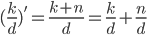
Notice that if we subtract from both sides we end up with

   (eq. 1)

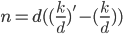
The quantity on the left is simply the difference between the old KD and the new KD.  Essentially, it’s the how much your KD changes if you add kills. Let's call that

So, a change in KD from adding kills is

This is interesting because the change is completely independent of your total kills, and only depends on your total deaths.* The dependence is one of the reasons why your KD seems to slowly creep along as you play more (and rack up more deaths). Of course, there are other factors too such as the fact that people don't actually get better at the game at a constant rate for as long as they play, but that's the topic of another discussion.


KD


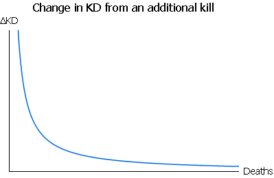
Kind of scary, isn't it! So, the TL;DR is:

The more deaths you have, the less you gain in KD from killing someone.


You can use this information to easily figure out how many kills you need to get (without dying!) to reach a new target KD.  Simply solve eq. 1 for :

Or, to write it in a way that's easier to read/ use, the number of kills you need () to reach a target KD is:

Again, notice the dependency on deaths.  As your deaths go up, so do the necessary number of kills needed to reach a given target KD.


*You may notice that if the d’s are all the same in eq. 1, you can cancel them out.  But this just leaves us with , telling us that the difference between the old kills and new kills is the number of kills you added, which is sort of obvious and not interesting. So leave the d's in there for now!


Pretty Graph of the Day

I ended up with this graph when doing some homework:

534HW2p3

It's the xy phase portrait of the system of differential equations as shown at the top of the figure.  There's a critical point at (0,0) and a limit cycle with radius . What a beauty!

The graph was made with pplane.