A Wild "import *" Appears

We all know that doing from foo import * in python is not good. Here's a specific instance I recently ran into which demonstrates how this can cause problems.

I was cleaning up some code, and decided to organize a decently sized list of imports (as outlined in the PEP8 style guide). To my surprise, simply changing the order of the imports broke the code. Scanning through the list, I spotted a from foo import * statement, which turned out to be causing problems.

Here's the setup:

File foo.py:

1 2	import datetime # do some stuff

File bar.py:

from datetime import datetime
from foo import *
# do some stuff
something = datetime.now() # code breaks here

When bar.py runs, an exception is thrown on line #4. What's happening is that the from foo import * statement is importing its datetime module, which is overriding the datetime class imported a line above. This means when you use datetime, you're actually using the module and not the class, as expected.

Science or Fiction Prediction: Getting a Statistical Edge

People sometimes say that if you're not sure what the answer is on a multiple choice question, you should guess c. I've always wondered if such a system could be applied to the Science or Fiction section on The Skeptic's guide to the Universe (SGU) podcast.

What a multiple choice test may look like

Quick background for non-listeners: The Skeptics Guide to the Universe is a super great science podcast that you should listen to. Each episode, they play a game called Science or Fiction, where one host (usually Steve) reads science news items or facts, one of which is completely made up. The others then try their best to determine which one is the fiction.

While it isn't practical to examine all of the multiple choice tests that have ever existed to determine if c is more likely to be correct, we can actually take a look at each round of Science or Fiction. It turns out that they keep good show notes on the SGU's website, including each science or fiction item and whether or not it's true.

As of this post, there are 480 episodes, so it's not practical to get the data by hand, but since each episode's page is neatly organized on the website it only took a couple minutes to whip up a little scraping script with python and Beautiful Soup to get the data. (Interestingly enough, scraping through all of the pages I found a tiny mistake: Item #1 of episode 247 is missing a "1". This broke my scraper the first time through.)

I only collected information about episodes where there were three science or fiction items (which is most of them), so that we can make a meaningful comparison:

	Item 1	Item 2	Item 3
Frequency	128	119	133
Probability of Fiction	33.7%	31.3%	35.0%

So it appears that item 2 is fiction less often than items 1 and 3. The question is, is it a "real" difference, or is it just part of the expected statistical background noise? Basically, we're trying to empirically determine if Steve uses some sort of random number generator to determine which item will be the fiction each week. Doing a chi squared test tells us that there's a 67% chance of observing such a difference.

In other words: the frequencies are consistent with a uniform distribution, and you can't get a significant edge based on the item ordering. Steve outsmarts us again!

I did the data collection and analysis with ipython, and you can check out the code here.

More Fun with OCN Server Data

This is a follow up to the previous post about tracking Overcast Network's (OCN) server activity.

A couple things:

At the time of that posting, there were only a few days of data in the database. Since then, the script has been churning away for the past few weeks, giving us a much larger sample.
The original scripts spend most of the time juggling dictionaries and reshaping the data to plot. This isn't particularly elegant. This time around I'm using Pandas for the data preprocessing after restructuring the database.

In retrospect, it would have probably made more sense to store the information in an SQL database. I used MongoDB only because I had never used it before (my favorite reason), and the prospect of being able to dump python dictionaries right in seemed fun. And I pretty much did just that - dumping dictionaries of data - which seemed simple enough at the time but ultimately led to processing complications later (see above).

With all of this in mind, I played with the data a bit in an ipython notebook, and so it only makes sense to display the code and results using the very cool browser notebook viewer. Check them out here! (If you aren't using the ipython notebook daily, you're blowing it. It's a lot of fun.)

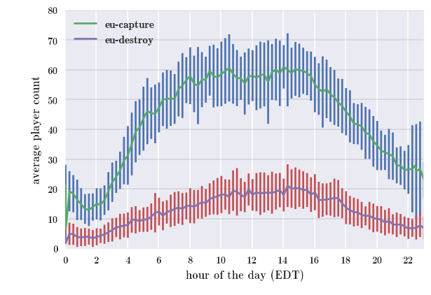
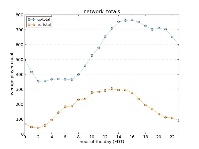
As you can see from the plots, the player count varies quite a bit throughout the day, even with a very large spread of players across the globe. This can cause some issues since many of the servers are designed with a certain number of players in mind. OCN recently implemented dynamic servers, which turn on and off depending on the number and distribution of players online and will hopefully solve this issue.

Code and more graphs

Tracking Overcast Network's Player Count with Python

Python quickie! Overcast Network is a large minecraft network and they have a lot of servers. They don’t keep track of the player count on all of these servers over time, so to assess the popularity of the different servers I wrote some scripts to collect server data and plot the results.

The collection script runs every 15 minutes via cron, grabs data from the play page and dumps it in a mongoDB database. The plotting class gets the data from the database and does a bunch of data maneuvering so it’s easy to work with (I should probably learn how to use data frames at some point) and then plots it with matplotlib:

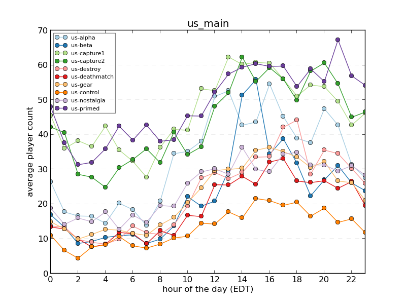
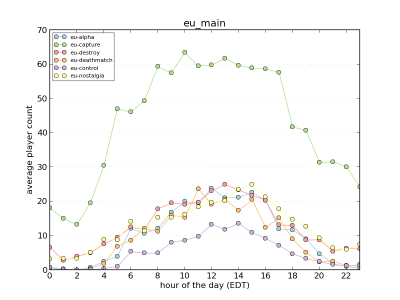
These plots show the average player activity per day (in one hour bins). There are only a few days worth of data shown here, which explains why the points tend to jump around a lot. As more data is collected, things should smooth out a bit. You can see more plots here.

Source

Related server tracking:

http://mc.ttaylorr.com/

New project: GG!

GG! Good game! This little web app was my Sunday project. It collects data and computes some basic statistics for Minecraft player-vs.-player minigame matches on the Overcast Network servers. It's still very much a work in progress, but check it out! Also, see the project on GitHub.

Simple LaTeX Table Generator

Anyone who's ever had to type up a large table in LaTeX knows that it can be a bit of work. When faced with a particulalry large table myself, I of course thought "why not python?".

It turns out there are already a few ways to generate latex tables, but here's my take:

""" This short script converts a CSV table into latex table.
 
Command Line Arguments:
 
required positional arguments:
infile input file name
 
optional arguments:
-h, --help show this help message and exit
-ncols N, --numbercolumns N
number of columns in file
-vd, --verticaldivider
adds vertical dividers to table
-hd, --horizontaldivider
adds horizontal dividers to table
"""
 
import csv
import sys
import argparse
 
# define and parse input arguments
parser = argparse.ArgumentParser()
parser.add_argument("infile", help="input file name")
parser.add_argument("-ncols", "--numbercolumns", type=int, help="number of columns in file", default=2)
parser.add_argument("-vd", "--verticaldivider", action="store_true", help="adds vertical dividers to table")
parser.add_argument("-hd", "--horizontaldivider", action="store_true", help="adds horizontal dividers to table")
args = parser.parse_args()
 
# csv input and latex table output files
infile = args.infile
outfile = infile +".table"
 
with open(infile, 'r') as inf:
    with open(outfile, 'w') as out:
        reader = csv.reader(inf)
 
        # build the table beginning code based on number of columns and args
        # columns all left justified
        code_header = "\\begin{tabular}{"
        for i in range(args.numbercolumns):
            code_header += " l "
            if i < args.numbercolumns - 1 and args.verticaldivider:
                code_header += "|"
        code_header += "}\n\\hline\n"
        out.write(code_header)
 
        # begin writing data
        for row in reader:
            # replace "," with "&"
            if args.horizontaldivider:
                out.write(" & ".join(row) + " \\\\ \\hline\n")
            else:
                out.write(" & ".join(row) + " \\\\ \n")
 
        if not args.horizontaldivider:
            out.write("\\hline\n")
 
        out.write("\\end{tabular}")

Example input file:

1,2,3
4,5,6

Running with the -vd and -hd flags to specify vertical and horizontal dividers produces:

\begin{tabular}{ l | l | l }
\hline
1 & 2 & 3 \\ \hline
4 & 5 & 6 \\ \hline
\end{tabular}

It's very minimal, and the main idea is that it does 95% of the work for you, leaving only very minor cosmetic tweaks.

Custom PBS qstat output

I recently became slightly annoyed with the information being displayed by PBS's qstat command. My main issue was that a simple qstat tends to cut off job names, which are very important if you're running multiple jobs with long, similar names that can't be distinguished when trimmed. The other extreme, qstat -f, prints way too much information that's difficult to efficiently navigate through.

There's probably an option flag that's midway between the two, but it seemed like a fun idea to write a simple intercepting script that only printed a couple things I found useful.

First, here's the first few lines of one job from the output of qstat -f to give you an idea of what the script is working with:

Job Id: 54314.master.localdomain
    Job_Name = df-AC6hex-N2-h2-HSE1PBE-opt-gdv
    Job_Owner = bw@master.localdomain
    resources_used.cput = 113:03:48
    resources_used.mem = 3177372kb
    resources_used.vmem = 4856612kb
    resources_used.walltime = 118:20:42
    job_state = R
    queue = verylong
    ...

In the output, each job is separated by a blank line. So, here's a python script that strips away some of the unneeded info, while printing the full job name:

#! /usr/bin/python
 
import subprocess
 
# get user name
user = subprocess.check_output(['whoami']).strip()
# get all jobs data
out = subprocess.check_output(['qstat','-f'])
lines = out.split('\n')
 
# build list of jobs, each job is a dictionary
jobs = []
for line in lines:
    if "Job Id:" in line:  # new job
        job = {}
        s = line.split(":")
        job_id = s[1].split('.')[0].strip()
        job[s[0].strip()] = job_id
    if '=' in line:
        s = line.split("=")
        job[s[0].strip()] = s[1].strip()
    elif line == '':
        jobs.append(job)
 
# print out useful information about user's jobs
print "\n   " + user + "'s jobs:\n"
for job in jobs:
    if job['Job_Owner'].split('@')[0] == user:        
        print "   " +  job['Job_Name']
        print "   Id: " + job['Job Id']
        print "   Wall time: " + job['resources_used.walltime']
        print "   State: " + job['job_state']
        print

Snippet of example output:

   bw's jobs:

   df-AC6hex-N2-h2-HSE1PBE-opt-gdv
   Id: 54314
   Wall time: 118:20:42
   State: R

   df-AC6hex-N2-h1b-HSE1PBE-opt-gdv
   Id: 54317
   Wall time: 118:13:38
   State: R

   df-AC6hex-N2-h2b-HSE1PBE-opt-gdv
   Id: 54321
   Wall time: 118:13:39
   State: R

   ...

The output of the command qstat -f is captured by python via the subprocess.check_output() function and organized into a dictionary, which allows for easy customization of what's printed out. After that, it's just some basic string processing and printing. Note also that it only prints information about the jobs of the user who is running the script.

electron exchange

holding the universe together

python