Tracking Overcast Network's Player Count with Python

Python quickie! Overcast Network is a large minecraft network and they have a lot of servers. They don’t keep track of the player count on all of these servers over time, so to assess the popularity of the different servers I wrote some scripts to collect server data and plot the results.

The collection script runs every 15 minutes via cron, grabs data from the play page and dumps it in a mongoDB database. The plotting class gets the data from the database and does a bunch of data maneuvering so it’s easy to work with (I should probably learn how to use data frames at some point) and then plots it with matplotlib:

These plots show the average player activity per day (in one hour bins). There are only a few days worth of data shown here, which explains why the points tend to jump around a lot. As more data is collected, things should smooth out a bit. You can see more plots here.

Source

Related server tracking:

http://mc.ttaylorr.com/

Minecraft Physics: Steve in Drag

An object falling under constant acceleration travels a distance in an amount of time given by

where is the object's starting velocity. For an object dropped from rest, . Plugging that in and solving for , we find

(1)

Using this equation, we can approximate the acceleration due to gravity in Minecraft by timing how long it takes something to fall some distance. This model assumes constant acceleration, which means it ignores things like drag forces from air resistance. It turns out, Minecraft actually does have air resistance, but we will get there a bit later.

Youtuber nopefully used the above approximation to determine the gravitational acceleration of sand blocks (further analyzed here). Since then, though, the addition of command blocks and scoreboards provide a simple way to time things in game, so that's the approach I'll take.

Experiment

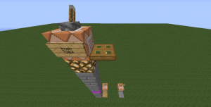
Figure 1: The dropper platform.

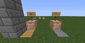
Figure 2: Timer stop and reset. The clock circuit is in the background.

The experiment is simple: jump off of stuff, time it with command blocks, and plug the result in the above equation (1) to figure out the gravitational acceleration of a player. For timing, I used Sethbling's stopwatch design. The timer-starting command block (figure 1) is activated by a lever which also triggers a trapdoor, causing you to fall onto a pressure plate below, stopping the timer (figure 2).

I repeated this experiment five times at three different heights. The data is in the table below (remember, a Minecraft block is 1 meter on each side):

Table 1: Results
Height (m)	Average Fall Time (s)	Acceleration (m/s²)
10	0.94	22.63
20	1.34	22.28
40	1.88	22.63

So using model (1), Minecraft's gravitational acceleration is around 23 m/s². But as I mentioned above, we're neglecting air resistance. There isn't an easy way to experimentally measure the air resistance, but luckily a video game provides us with something that nature does not: the source code. So let's cheat a little bit and take a look under the hood.

Cheating

In the EntityLivingBase class, there's a method named moveEntityWithHeading that is called 20 times per second (each "tick"), updating the entity's velocity. If there isn't a block under the living entity (in other words, it's falling), the downward velocity is increased by 0.08 and decreased by 2% each tick. This means there's a constant acceleration component that is 0.08 blocks/tick² = 32 m/s² and a drag force that is directly proportional to the velocity. 32 m/s² is a lot different than our measured 23 m/s², so clearly the drag force is not something that can be ignored. Also, 32m/s² is over 3 times greater than the gravity on Earth! (An inventory of cobble is seriously heavy.)

On Earth, the gravitational acceleration is about 9.8m/s² near the surface, and is the same for all objects regardless of how much they weigh. This isn't the case in Minecraft, as you can see in the more detailed table on Minecraft wiki. The "drag" contribution is also different for different entities (which is slightly more realistic since air resistance depends on the size and shape of the object).

Fluid Dynamics

The existence of a non-negligible drag force complicates the task of experimentally determining Minecraft's gravitational acceleration. But it also means that we have a more fun differential equation to play with! We can start out by writing down the equations of motion for the object falling. From the source code, we know that the drag force is proportional to the velocity, so we can use a linear drag model for the forces:

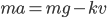
where is the object's mass, is the total acceleration, is the acceleration due to gravity, is some sort of drag coefficient and is the object's velocity. Remembering from physics class that acceleration is the first derivative of velocity with respect to time (denoted ), we can substitute . Doing that and diving both sides by gives us an equation for the total acceleration:

The value of is what's in the "Drag" column in the Minecraft wiki table. Solving for the velocity as a function of time, we find

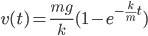(2)

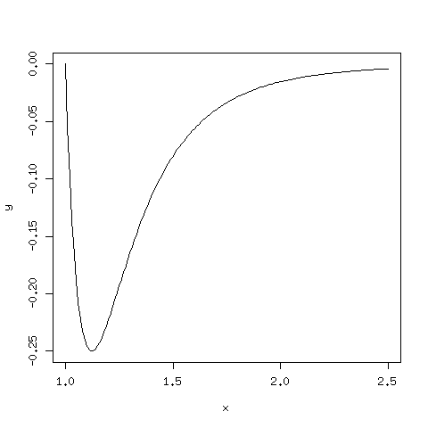
We can take some values of and from the table and graph the velocity (equation 2) of each of the different entities as they fall:

The velocity increases for a bit, but the rate at which it increases (the acceleration) slows with time until the entity travels at a constant velocity. This is called terminal velocity, and it's reached when the gravitational force and the force due to air resistance balance out. You can see that a falling player can catch up to most other entities, except for fired arrows.*

You can see the raw data in a Google spreadsheet here. I encourage you to try out this set up and Minecraft physics experiments. Please share your findings!

*So if, for example, you're engaging in a PvP fight on Overcast Network and someone tries to jump out of the world to deny you a kill, look over the edge and shoot! Your arrow has a chance of catching up to them.

Minecraft Minigame Match Dynamics

As a physics student, it can be difficult to not think of things as point particles - even players engaging in minecraft minigame matches on the Overcast Network.

So as a Saturday afternoon project, I made a simple client mod that allows you to write all of the player positions on the current world to a CSV file. Then, using Mathematica, I processed the data and made some simple visualizations:

This shows the player positions, colored by team. This match takes place on a map called Warlock (one of my favorites), and the goal is to be the first team to break the other team's monument (which is made out of two pieces of obsidian). Red team won this match, and you can see a red guy sneaking near the blue's monument (probably underground) in the bottom left for a few minutes before finally breaking it.

See more visualizations here (I don't want to lag up the page with gifs), and view the source code here.

Lennard R. Jones

I started learning a bit of R recently at a data processing workshop. I'm enjoying it so far. Sometimes it's nice to see what else is "out there" (as in, not python).

One interesting thing is the fact that many arithmetic operations on vectors are treated element-wise. So for example, adding two vectors with "+" just adds the corresponding elements. This can be useful for generating some quick function plots in very few lines and with no need for explicit loops or anything like that.

Here's a simple plot of the Lennard-Jones potential as you would create it in an interactive R session:

1
2
3

x <- seq(0,2.5,0.01)    # generate grid from 0 to 2.5 in steps of 0.01
y <- x^(-12) - x^(-6)   # evaluate Lennard-Jones potential on all grid points
plot(x,y,type="l")      # plot with a line

Of course, you can get fancier and create beautiful plots with R, but it's also nice for quick-and-dirty visualizations.

Pretty Graph of the Day, Part II

I like this series of graphs because it looks like someone is pulling on the solution like it's a string, until SNAP! What's being shown here is the numerical solution to the initial value problem

, , .

As you might suspect from the denominator, there's trouble when . This results in a problem that's not well-posed. Using the same numerical scheme but only a different number of grid points produces wildly different behaviors. What's basically happening is that if the numerical scheme hits the trouble region "just right" due to the grid point spacing, the gigantic derivative sends the solution flying off to some large and incorrect value.

You can reproduce this figure in Mathematica with the following code:

(* 4th Order Runge-Kutta Method *)
rungeKutta[y0_, npoints_, a_, b_, f_] := (
   h = (b - a)/(npoints - 1);
   y = Table[0, {npoints}];
   t = Table[0, {npoints}];
   y[[1]] = y0;
   t[[1]] = a;
   Do[
    yn = y[[n]];
    tn = t[[n]];
    m1 = f[tn, yn];
    m2 = f[tn + 0.5*h, yn + 0.5*h*m1];
    m3 = f[tn + 0.5*h, yn + 0.5*h*m2];
    m4 = f[tn + h, yn + h*m3];
    y[[n + 1]] = yn + (1/6)*h*(m1 + 2*m2 + 2*m3 + m4);
    t[[n + 1]] = tn + h;
    , {n, 1, npoints - 1}];
   solution = Table[{t[[i]], y[[i]]}, {i, 1, Length[t]}];
   Return[solution];
   );
 
 f[t_, y_] := 1/(y - 1)^2
y0 = 0;
a = 0; (* Starting t *)
b = 1; (* Ending t *)
 
rks = {};
Do[
  npoints = 10^5 + i; (* Number of grid points *) 
  sol = rungeKutta[y0, npoints, a, b, f];
  p = ListPlot[sol, PlotStyle -> {PointSize[0.001] , Orange}, 
    Frame -> True, AxesLabel -> {"t", "y"}, 
    PlotLabel -> 
     "10^5+ " <> ToString[i] <> 
      " grid points"];
  AppendTo[rks, p];
  , {i, 0, 4}];
 
GraphicsColumn[Table[rks[[j]], {j, 5}], Frame -> All, ImageSize -> 300]

It'll probably take several seconds to run because of the large number of grid points used in each solution.

Pretty Graph of the Day

I ended up with this graph when doing some homework:

534HW2p3

It's the xy phase portrait of the system of differential equations as shown at the top of the figure. There's a critical point at (0,0) and a limit cycle with radius . What a beauty!

The graph was made with pplane.

electron exchange

holding the universe together

graph